Detailed worked example • gamlss.longitudinal

This vignette shows an end-to-end workflow for fitting a simulated longitudinal dataset with a longitudinal gamlss model with gamlss margins and copula dependence using gamlss.longitudinal.

The example is simulated so that we can compare the fitted model with the known truth, but the same workflow is intended for a real dataset (excluding simulation of the dataset, of course).

The workflow is:

Simulate a longitudinal dataset using builtin helper simulate_longitudinal_dataset()
Inspect the marginal response, covariates, missingness, and pairwise dependence,
Select a marginal distribution and copula family,
Fit the longitudinal model incuding covariate selection,
Review the final model fit,
Answer applied questions with prediction, marginal effects, simulation, and benchmark comparisons.

For simplicity, a number of decisions on covariate structure are shortened based on the known structure of the underlying data with some illustrative comparisons between alternatives, however in an unknown data context of course a large number of alternative covariate structures may be tested.

First we load required packages for this vignette:

library(gamlss.longitudinal)
library(ggplot2)

For installation of gamlss.longitudinal, use remotes::install_github("ahibbert/gamlss.longitudinal").

Simulate data

We simulate a longitudinal dataset with 120 subjects with observations at 5 time points. The simulated response is generalized gamma (GG()) distributed with skewed low-value correlation between time points generated using a Clayton copula. A 10% response missingness is applied at random.

We also include the following covariates:

a three-level treatment group: control, low, or high;
a subject-level age generated uniformly between 25 and 70;
a repeated observation time scaled to [0, 1].

Simulation code

set.seed(20260521)

n_subject <- 120
time_points <- seq(0, 1, length.out = 5)

treatment_effect <- c(control = 0, low = 0.30, high = 0.65)

truth_mu_age_smooth <- function(x) {
  sim_smooth_bump(x, amplitude = 0.60, location = 0.62, width = 0.18) +
    sim_smooth_sin(x, amplitude = 0.16)
}

truth_sigma_age_smooth <- function(x) {
  sim_smooth_u(x, amplitude = 0.45)
}

truth_theta_age_smooth <- function(x) {
  sim_smooth_bump(x, amplitude = 1, location = 0.45, width = 0.22)
}

dat <- simulate_longitudinal_dataset(
  n = n_subject,
  times = time_points,
  margin_dist = GG(mu.link = "log", sigma.link = "log", nu.link = "identity"),
  copula_dist = "C",
  covariates = function(base) {
    simulate_longitudinal_covariates(
      base,
      subject = list(
        treatment = function(subject_data) {
          factor(
            sample(c("control", "low", "high"), nrow(subject_data), replace = TRUE),
            levels = c("control", "low", "high")
          )
        },
        age = function(subject_data) stats::runif(nrow(subject_data), 25, 70)
      ),
      observation = list(
        time_scaled = function(long_data) sim_rescale01(long_data$time)
      )
    )
  },
  margin_params = list(
    mu = function(d) {
      age_scaled <- sim_rescale01(d$age)
      eta_mu <- 1.00 +
        sim_factor_effect(d$treatment, treatment_effect) +
        0.35 +
        truth_mu_age_smooth(age_scaled)
      exp(eta_mu)
    },
    sigma = function(d) {
      age_scaled <- sim_rescale01(d$age)
      eta_sigma <- -1.05 +
        0.25 * sim_factor_effect(d$treatment, c(control = 0, low = 1, high = 1)) +
        1.25 * d$time_scaled +
        truth_sigma_age_smooth(age_scaled)
      exp(eta_sigma)
    },
    nu = function(d) {
      age_scaled <- 
      1.15 + 0.55
    }
  ),
  copula_params = list(
    theta = function(e) {
      age_scaled <- sim_rescale01(e$age)
      time_left_scaled <- sim_rescale01(e$time_left)
      eta_theta <- -0.70 +
        1.80 * time_left_scaled +
        truth_theta_age_smooth(age_scaled)
      exp(eta_theta)
    }
  ),
  seed = 20260521
)

dat$age_scaled <- sim_rescale01(dat$age)

missing_weight <- stats::plogis(
  -0.70 +
    1.15 * dat$time_scaled +
    0.45 * (dat$treatment == "high") -
    0.30 * dat$age_scaled
)
missing_rows <- sample(
  seq_len(nrow(dat)),
  size = round(0.10 * nrow(dat)),
  replace = FALSE,
  prob = missing_weight
)
dat$response[missing_rows] <- NA_real_
dat$response_missing <- is.na(dat$response)

dataset=dat[,c("subject", "time", "response", "treatment", "age")]

Inspect the response

Our first check is to ensure the dataset is in the correct shape to ingest in the gamlss_longitudinal fit. The data should include:

one row per subject and time combination,
one column for each of the response, subject identifier and timepoint, and
timepoint should be an ordered factor (or will be automatically ordered using order()).

# Check data columns / subject/time counts
str(dataset)
#> 'data.frame':    600 obs. of  5 variables:
#>  $ subject  : Factor w/ 120 levels "1","2","3","4",..: 1 1 1 1 1 2 2 2 2 2 ...
#>  $ time     : num  0 0.25 0.5 0.75 1 0 0.25 0.5 0.75 1 ...
#>  $ response : num  14.063 12.732 5.384 NA 0.247 ...
#>  $ treatment: Factor w/ 3 levels "control","low",..: 3 3 3 3 3 2 2 2 2 2 ...
#>  $ age      : num  34.6 34.6 34.6 34.6 34.6 ...
table(dataset$treatment)
#> 
#> control     low    high 
#>     150     210     240
table(dataset$time)
#> 
#>    0 0.25  0.5 0.75    1 
#>  120  120  120  120  120

Since missingness and dropout in particular is common in longitudinal datasets, we include an internal helper to summarise overall missingness. check_missingness() summarises the missingness in the response overall then builds a simple logisitic regression for the response against included predictors to screen for any strong trends. This can be treated as an indicator of whether missingness at random can be reasonably assumed based on the included features, however it cannot rule out other factors that may be driving missingness. In this case, time is considered as related to missingness (i.e. dropout) but no other factors are found to be significant at p=0.05 which is the default for warnings.

missingness_check <- check_missingness(
  dataset,
  response_var = "response",
  time_var = "time",
  subject_var = "subject",
  predictors = c("time", "treatment", "age")
)

print(missingness_check)
#> 
#> Response Missingness Check
#> --------------------------
#>    n n_missing prop_missing
#>  600        60          0.1
#> 
#> Assessment: covariate_related_missingness 
#> Response missingness is associated with observed predictor(s): time . This is compatible with MAR conditional on the observed predictors, but it does not rule out MNAR.
#> 
#> Predictor tests:
#>       term statistic df p_value
#>       time    5.4370  1 0.01971
#>  treatment    5.7599  2 0.05614
#>        age    0.3881  1 0.53329

As these are longitudinal data, time is often a factor which may influence the shape of the joint distribution. We first briefly review the moments of the observed marginal distribution and the correlation structure against time to inform model selection. In this case, there is not a strong effect of time on the mean on initial inspection but there is clearly a trend in variance, skewness and kurtosis over time. Reviewing the pairwise correlation over time (the first off-diagonal), it appears there may also be a trend in increasing correlation for adjacent observations over time, with decreasing correlation with time-distance as is often common in longitudinal data.

aggregate(response ~ time, dataset, \(x) {
  x <- x[!is.na(x)]
  c(mean = mean(x),
    var = var(x),
    skew = mean((x - mean(x))^3) / sd(x)^3,
    kurt = mean((x - mean(x))^4) / sd(x)^4)
})
#>   time response.mean response.var response.skew response.kurt
#> 1 0.00     7.5026530   15.9464317     1.2445134     4.7531921
#> 2 0.25     6.1712956   13.6168051     0.9349299     3.3786179
#> 3 0.50     5.2590809   20.6433649     1.2684042     4.4610233
#> 4 0.75     5.4392198   57.3775583     2.5454634    10.0150800
#> 5 1.00     4.4063413   50.4118173     3.1359385    15.6310270

cor(reshape(dataset[c("subject", "time", "response")],
            idvar = "subject", timevar = "time", direction = "wide")[-1],
    use = "pairwise.complete.obs")
#>               response.0 response.0.25 response.0.5 response.0.75 response.1
#> response.0     1.0000000     0.4483821    0.4098473     0.3300501  0.1857214
#> response.0.25  0.4483821     1.0000000    0.6086610     0.4939688  0.1723208
#> response.0.5   0.4098473     0.6086610    1.0000000     0.6569918  0.2679377
#> response.0.75  0.3300501     0.4939688    0.6569918     1.0000000  0.5199290
#> response.1     0.1857214     0.1723208    0.2679377     0.5199290  1.0000000

We can also visually inspect the response and dependence between timepoints using the included helper plot_dist(). The function plots the marginal distribution for each time point on the negative diagonal then the normal-transformed pseudo-observations against one another to provide a view of the correlation between each pair of margins. It’s clear from the plots that:

there is increasing skewness / tail over time (see the negative diagonal),
the overall level of correlation increases with time (see row 1, col 2 versus row 4, col 5),
the shape of the correlation is skewed to low-value correlation (see row 4, col 5)

So this informs our model that it’s likely both the copula and marginal parameters (at least beyond the mean) will likely depend on time in some way. This can often be an important part of the distribution selection (see next section).

plot_dist(
  dataset,
  margin_dist = GG(mu.link = "log", sigma.link = "log", nu.link = "identity"),
  subject_var = "subject",
  time_var = "time",
  response_var = "response"
)

Matrix plot of marginal response distributions and dependence by time.

Choose a marginal distribution

The response here is continuous and positive. For any distribution we can use the function select_margin() to fit an intercept-only model to the response distribution and provide a ranked list of fits by likelihood criteria (default is AIC).

margin_selection <- select_margin(
  dataset,
  response_var = "response",
  time_var = "time",
  type = "realplus"
)

print(margin_selection)
#> 
#> Marginal Distribution Screen
#> ----------------------------
#> Selected: BCPEo 
#> 
#>  family      AIC     type     screen_model rank    delta_AIC
#>   BCPEo 2886.334 realplus pooled_intercept    1 0.000000e+00
#>    BCPE 2886.334 realplus pooled_intercept    2 1.066837e-09
#>     BCT 2888.053 realplus pooled_intercept    3 1.718650e+00
#>    BCTo 2888.053 realplus pooled_intercept    4 1.718650e+00
#>    BCCG 2892.121 realplus pooled_intercept    5 5.787225e+00
#>   BCCGo 2892.121 realplus pooled_intercept    6 5.787225e+00
#>     GB2 2902.372 realplus pooled_intercept    7 1.603843e+01
#>      GG 2929.585 realplus pooled_intercept    8 4.325148e+01
#>      GA 2954.450 realplus pooled_intercept    9 6.811586e+01
#>     GIG 2956.450 realplus pooled_intercept   10 7.011586e+01

The BCPEo is selected as the best fitting distribution as it is highly flexible and is able the capture the shape of the shared distribution. However, given we know that time is a strong component of the moments, the best model is likely to be using a marginal distribution which can change with time.

We can set the option time_intercepts=TRUE in select_margin() which allows each parameter of the marginal distribution to vary with time. This method then selects GG() and GA() as the best models by AIC. We will take these two distributions forwards as our two potential distributions for the final model, depending on whether the additional parameter for the GG() over the GA() adds sufficent fit to account for the additional degrees of freedom consumed.

margin_selection <- select_margin(
  dataset,
  response_var = "response",
  time_var = "time",
  type = "realplus",
  time_intercepts = TRUE
)

margin_selection
#> 
#> Marginal Distribution Screen
#> ----------------------------
#> Selected: GA 
#> 
#>  family      AIC     type    screen_model pooled_AIC converged rank  delta_AIC
#>      GA 2687.496 realplus time_intercepts   2954.450      TRUE    1   0.000000
#>      GG 2694.061 realplus time_intercepts   2929.585      TRUE    2   6.565322
#>     GB2 2706.209 realplus time_intercepts   2902.372     FALSE    3  18.713260
#>    BCTo 2706.904 realplus time_intercepts   2888.053      TRUE    4  19.408152
#>     BCT 2706.904 realplus time_intercepts   2888.053      TRUE    5  19.408163
#>     WEI 2711.468 realplus time_intercepts   2970.726      TRUE    6  23.972717
#>    WEI3 2711.468 realplus time_intercepts   2970.726      TRUE    7  23.972726
#>    WEI2 2711.474 realplus time_intercepts   2970.726      TRUE    8  23.977945
#>  LOGNO2 2803.629 realplus time_intercepts   3364.255      TRUE    9 116.133256
#>   LOGNO 2803.629 realplus time_intercepts   3364.255      TRUE   10 116.133256
#> 
#> Warning: one or more printed time-intercept marginal fits did not report convergence.

We can review the fitted margin over the overall distribution using plot_margin_fit().

For illustration we’ll compare the fit without time-varying intercepts to the fit with time-varying intercepts.

First let’s review the fit without time intercepts.

margin_overlay_plots <- list(
  plot_margin_fit(
    dataset,
    margin_dist = GA(),
    response_var = "response",
    bins = 30,
    time_var = "time",
    plot = FALSE
  )$plot,
  plot_margin_fit(
    dataset,
    margin_dist = GG(),
    response_var = "response",
    bins = 30,
    time_var = "time",
    plot = FALSE
  )$plot
)

ggpubr::ggarrange(plotlist = margin_overlay_plots, ncol = 2, nrow = 1)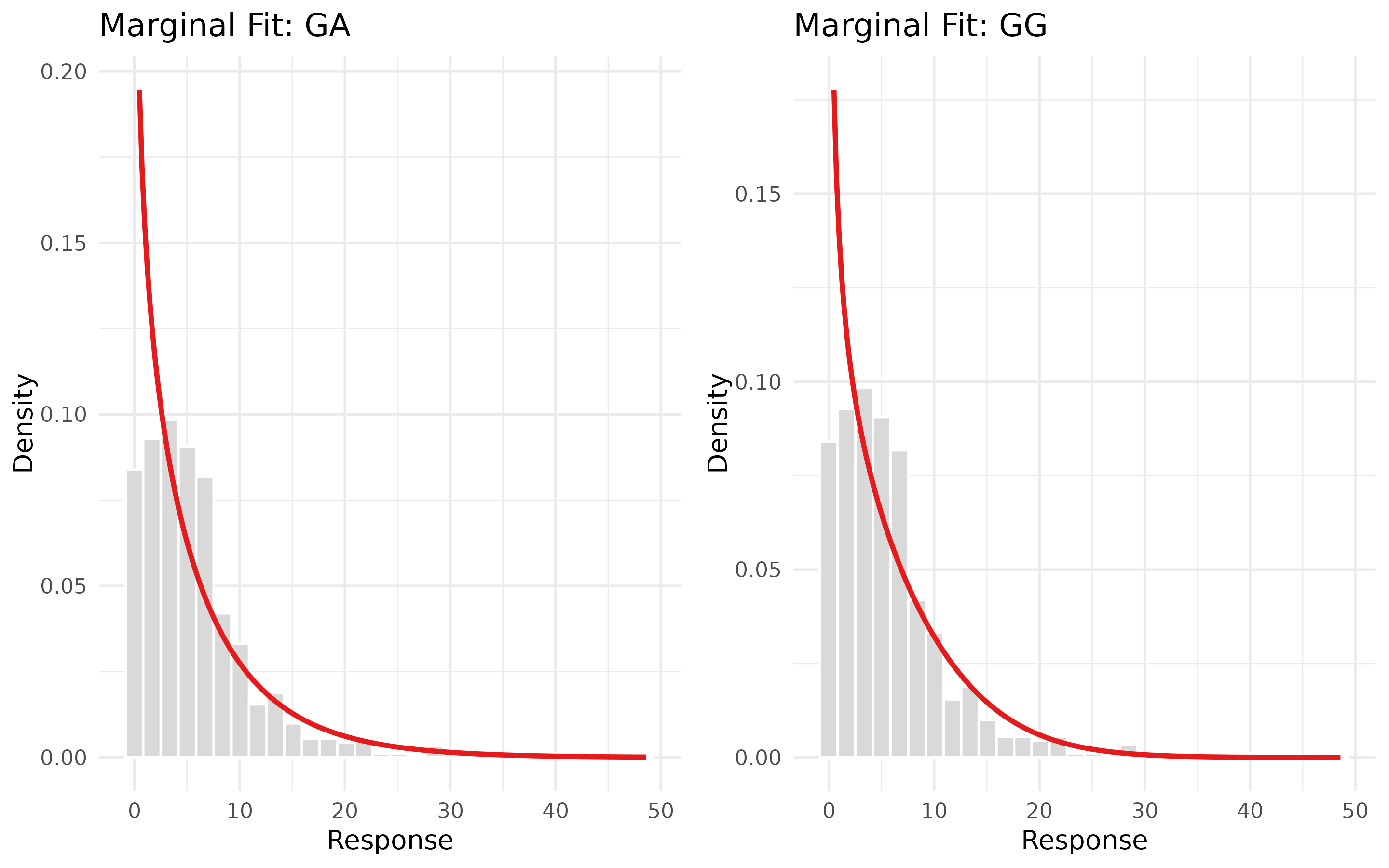

Histograms of observed responses comparing generalized gamma and gamma marginal fits without time-intercepts.

Clearly the GA() and GG() are not fitting well here, which is why the BCPE() was selected as the best non-time-varying model.

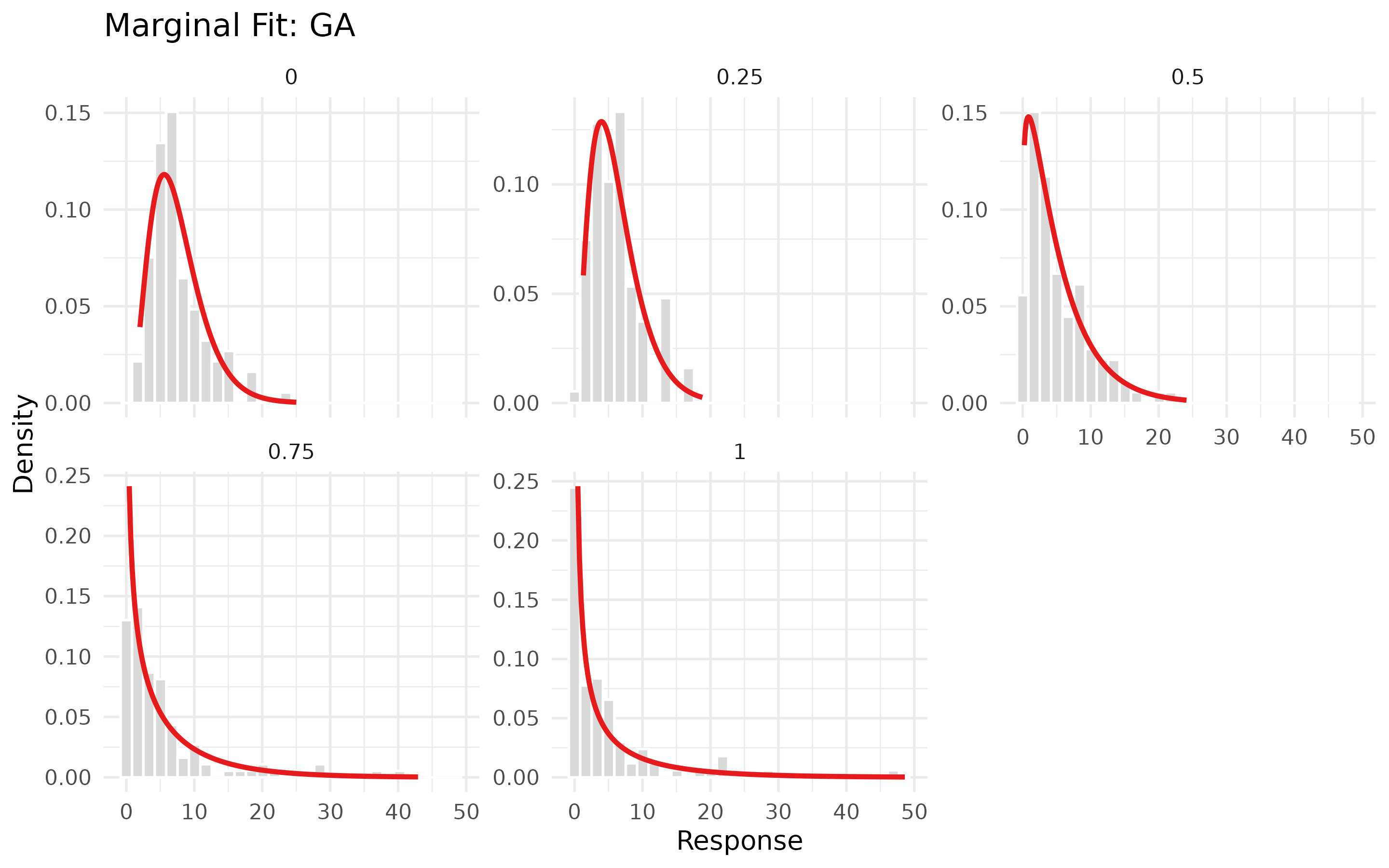
We can review the fits over time by selecting by_time=TRUE in plot_margin_fit. With this faceting, GA() and GG() closely follow the changing shape of the distribution over time as implied by the likelihood criteria. While it’s not a strong effect, it appears the GG() captures the extreme distributions at first and last timepoints slightly more accurately than the base GA() model, but both capture the changing shape of the distribution reasonably.

plot_margin_fit(
  dataset, 
  margin_dist = GA(), 
  time_intercepts = TRUE, 
  by_time = TRUE, 
  time_var ="time", 
  response_var = "response"
)

Histograms of fitted GA with time-varying intercepts for each parameter.

plot_margin_fit(
  dataset, 
  margin_dist = GG(),
  time_intercepts = TRUE,
  by_time = TRUE,
  time_var = "time",
  response_var = "response"
)

Histograms of fitted GG with time-varying intercepts for each parameter.

Choose a copula family

Once we have a starting fit for the margin, we can select a copula distribution. The copula distribution depends on the shape of the margin so the margin must be selected first. We do provide the option for choosing both margin and copula jointly using select_joint_distribution() however this is quite a slow fit, and generally does not select differently to the much faster process using select_margin() followed by select_copula(). Instead we would suggest sensitivity / alternative testing for a final selection of margins or copulas, or for the final fitted model, rather than spending compute time at the early stage before covariates are selected.

select_copula() asseses available copula fits by likelihood criteria for the starting marginal model. The copula is fit on pseudo-observations which have been created using the marginal fit. The user can either pass in the best model from select_margin() using margin_dist=margin_selection or can specify a marginal fit with margin_dist and time_intercepts=TRUE/FALSE. If the user really wants, they can also fully specify a gamlss.longitudinal model with formulas for all the intercepts and select a copula that way, however we would suggest this as a final sensitivity test rather than at this stage since covariates are not yet reviewed.

As dependence structure can also shift with time, we also provide the option to provide time-based intercepts in the select_copula() function using copula_time_intercepts=TRUE in case the changing shape over time selects a different copula family than a static single parameter as was the case for marginal parameters.

We provide selection here for GA() (using margin_dist=margin_selection) and GG() (directly specifying margin_dist and time_intercepts) with both time-varying and non-time-varying copula paramter.

In this case, the best fitting copula is Clayton both with and without a time covariate for the copula parameter. All four options select the Clayton copula so we move forward with this.

copula_selection <- select_copula(
  data = dataset,
  response_var = "response",
  margin_dist = margin_selection,
  subject_var = "subject",
  time_var = "time"
)
print(copula_selection)
#>   family       par par2       tau    logLik       AIC       BIC n_pairs
#> 1      t 0.6994834    6 0.4931730 136.22365 -268.4473 -260.4946     394
#> 2      C 1.5331365    0 0.4339307 132.78513 -263.5703 -259.5939     394
#> 3      N 0.6926152    0 0.4870831 129.73924 -257.4785 -253.5021     394
#> 4      F 5.7673936    0 0.5017071 122.51872 -243.0374 -239.0611     394
#> 5      G 1.8307929    0 0.4537886 110.49402 -218.9880 -215.0117     394
#> 6      J 1.9420289    0 0.3419512  71.33603 -140.6721 -136.6957     394

copula_selection <- select_copula(
  data = dataset,
  response_var = "response",
  margin_dist = margin_selection,
  subject_var = "subject",
  time_var = "time",
  copula_time_intercepts = TRUE
)
print(copula_selection)
#>   family par par2       tau    logLik       AIC       BIC n_copula_time_levels
#> 1      C  NA    0 0.4431982 149.95523 -291.9105 -276.0050                    4
#> 2      t  NA   NA 0.5014935 151.52320 -287.0464 -255.2356                    4
#> 3      N  NA    0 0.4949967 145.08277 -282.1655 -266.2601                    4
#> 4      F  NA    0 0.5017947 136.17264 -264.3453 -248.4399                    4
#> 5      G  NA    0 0.4548704 120.62797 -233.2559 -217.3505                    4
#> 6      J  NA    0 0.3472754  78.31384 -148.6277 -132.7223                    4
#>   n_pairs
#> 1     394
#> 2     394
#> 3     394
#> 4     394
#> 5     394
#> 6     394

copula_selection <- select_copula(
  data = dataset,
  response_var = "response",
  margin_dist = GG(),
  time_intercepts = TRUE,
  subject_var = "subject",
  time_var = "time"
)
print(copula_selection)
#>   family       par par2       tau   logLik       AIC       BIC n_pairs
#> 1      t 0.6908198    4 0.4855004 137.0033 -270.0067 -262.0540     394
#> 2      C 1.5312958    0 0.4336357 132.6829 -263.3657 -259.3894     394
#> 3      N 0.6929039    0 0.4873380 129.9614 -257.9229 -253.9465     394
#> 4      F 5.7633204    0 0.5014841 122.2383 -242.4766 -238.5003     394
#> 5      G 1.8389989    0 0.4562259 111.9140 -221.8281 -217.8517     394
#> 6      J 1.9600796    0 0.3460953  73.0801 -144.1602 -140.1839     394

copula_selection <- select_copula(
  data = dataset,
  response_var = "response",
  margin_dist = GG(),
  time_intercepts = TRUE,
  subject_var = "subject",
  time_var = "time",
  copula_time_intercepts = TRUE
)
print(copula_selection)
#>   family par par2       tau    logLik       AIC       BIC n_copula_time_levels
#> 1      C  NA    0 0.4451424 152.93507 -297.8701 -281.9647                    4
#> 2      t  NA   NA 0.5024956 152.81188 -289.6238 -257.8130                    4
#> 3      N  NA    0 0.4950534 144.72822 -281.4564 -265.5510                    4
#> 4      F  NA    0 0.5015021 136.22741 -264.4548 -248.5494                    4
#> 5      G  NA    0 0.4578189 121.54984 -235.0997 -219.1943                    4
#> 6      J  NA    0 0.3507796  79.20618 -150.4124 -134.5070                    4
#>   n_pairs
#> 1     394
#> 2     394
#> 3     394
#> 4     394
#> 5     394
#> 6     394

copula_selection <- select_copula(
  data = dataset,
  response_var = "response",
  margin_dist = GG(),
  subject_var = "subject",
  time_var = "time",
  time_intercepts = TRUE,
  copula_time_intercepts = TRUE
)
print(copula_selection)
#>   family par par2       tau    logLik       AIC       BIC n_copula_time_levels
#> 1      C  NA    0 0.4451424 152.93507 -297.8701 -281.9647                    4
#> 2      t  NA   NA 0.5024956 152.81188 -289.6238 -257.8130                    4
#> 3      N  NA    0 0.4950534 144.72822 -281.4564 -265.5510                    4
#> 4      F  NA    0 0.5015021 136.22741 -264.4548 -248.5494                    4
#> 5      G  NA    0 0.4578189 121.54984 -235.0997 -219.1943                    4
#> 6      J  NA    0 0.3507796  79.20618 -150.4124 -134.5070                    4
#>   n_pairs
#> 1     394
#> 2     394
#> 3     394
#> 4     394
#> 5     394
#> 6     394

If the user wishes to compare a few combinations of fits for overall joint distribution, this is a reasonable point to confirm using select_joint_distribution(). For example, let’s compare the GA, GG and a benchmark standard normal NO, and compare fits for N and C copulas with time intercepts for both margin and copula fits. This takes about 30 seconds to run for this example. The selected joint fits are GA+C as the best AIC/BIC and GG+C as the best log likelihood which agrees with the previous process.

joint_selection <- select_joint_distribution(
  data = dataset,
  response_var = "response",
  subject_var = "subject",
  time_var = "time",
  time_intercepts = TRUE,
  copula_time_intercepts = TRUE,
  margin_families = c("GA", "GG", "NO"),
  copula_families = c("N", "C")
)

print(joint_selection)
#> 
#> Joint Distribution Screen
#> -------------------------
#> Selected: GA+C 
#> Criterion: AIC 
#> 
#>  rank margin_family copula_family    logLik      AIC      BIC EDF converged
#>     1            GA             C -1180.985 2389.971 2451.528  14      TRUE
#>     2            GG             C -1176.935 2391.870 2475.412  19     FALSE
#>     3            GG             N -1179.337 2396.673 2480.215  19      TRUE
#>     4            GA             N -1187.644 2403.288 2464.845  14      TRUE
#>     5            NO             C -1455.730 2939.460 3001.017  14      TRUE
#>     6            NO             N -1566.724 3161.448 3223.005  14      TRUE
#>  elapsed_sec error
#>     3.606573  <NA>
#>    10.936026  <NA>
#>     7.137297  <NA>
#>     1.607073  <NA>
#>     5.047800  <NA>
#>     3.017524  <NA>
#> 
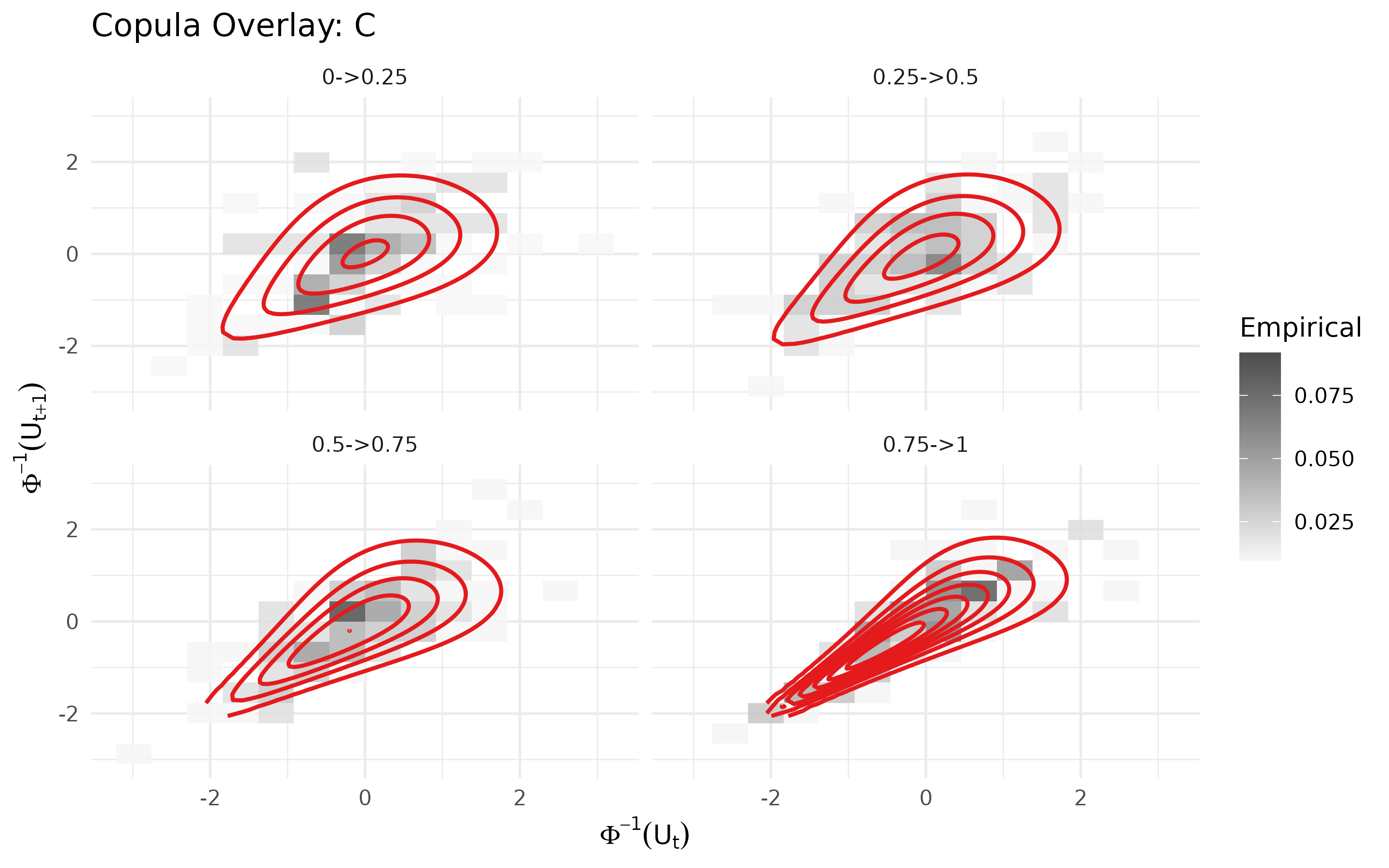
#> Warning: one or more printed joint candidate fits did not report convergence.

We can now review the copula fit visually using plot_copula_fit. The updated fit appears to accurately capture the low-dependence shape of the data as well as the increasing correlation over time.

plot_copula_fit(
  dataset,
  margin_dist = margin_selection,
  copula_dist = copula_selection,
  subject_var = "subject",
  time_var = "time",
  response_var = "response",
  by_time = TRUE,
  bins=14
)

Fit The Longitudinal Model

Model fitting for gamlss.longitudinal should always follow the parameter heirarchy for the margin, mu -> sigma -> nu -> tau, and for the copula theta -> zeta. There is not a strict heirarchy between marginal versus copula paramters as copula parameters can affect the standard errors for the margin, resulting in different parameters being significant in the margin, and marginal parameters can affect the copula fit so the process is necessarily iterative. However, in general it is reasonable to get a good fit for the margin with the most significant factors before iterating on covariate fits for the copula parameter. Following a strict margin before copula process will generally yield similar results, though may result in removing some previously significant factors (or adding previously insiginficant factors) from the margin depending on the copula fit.

We will use the GG() fit to start for the additional flexibility for the additional parameter, and if it is not significant with an intercept or covariates then we can reduce the model the GA(). The selected copula was C under all margin settings so we will use this.

Let’s begin by inspecting a fully specified model with factor terms for time and treatment, and a smooth term for age on every covariate, including the copula parameter.

fit_fullyspecified <- gamlss_longitudinal(
  dataset = dat,
  margin_dist = GG(),
  copula_dist = "C",
  time_var = "time",
  subject_var = "subject",
  mu.formula = response ~ treatment + as.factor(time) + s(age),
  sigma.formula = ~ treatment + as.factor(time) + s(age),
  nu.formula = ~ treatment + as.factor(time) + s(age),
  theta.formula = ~ treatment + as.factor(time) + s(age)
)

summary(fit_fullyspecified)
#> 
#> GAMLSS Longitudinal Model Summary
#> --------------------------------
#> Margin distribution: GG 
#> Copula distribution: C 
#> Observations: 600  | Subjects: 120  | Time points: 5 
#> Fixed coefficients: 27  | Smooth terms: 4  | Smooth EDF: 10.6613 
#> VCOV: analytical  | Requested: analytical 
#> Hessian condition number: 135688 
#> 
#> Fixed coefficients:
#> --------------------
#>   [mu]
#>     term                                 estimate  std_error   p_value  signif
#>     mu.intercept                           1.6953     0.0601  <0.00001  ***   
#>     mu.treatmentlow                        0.2142     0.0923   0.02026  *     
#>     mu.treatmenthigh                       0.5960     0.1089  <0.00001  ***   
#>     mu.as.factor(time_covariate)0.25      -0.1848     0.0753   0.01407  *     
#>     mu.as.factor(time_covariate)0.5       -0.1396     0.0972   0.15087        
#>     mu.as.factor(time_covariate)0.75      -0.0247     0.1763   0.88840        
#>     mu.as.factor(time_covariate)1         -0.1632     0.6039   0.78690        
#>   --------------------
#>   [sigma]
#>     term                                 estimate  std_error   p_value  signif
#>     sigma.intercept                       -1.2832     0.1454  <0.00001  ***   
#>     sigma.treatmentlow                     0.4950     0.1038  <0.00001  ***   
#>     sigma.treatmenthigh                    0.3377     0.2825   0.23193        
#>     sigma.as.factor(time_covariate)0.25    0.2696     0.1295   0.03729  *     
#>     sigma.as.factor(time_covariate)0.5     0.6712     0.1525   0.00001  ***   
#>     sigma.as.factor(time_covariate)0.75    1.0371     0.1164  <0.00001  ***   
#>     sigma.as.factor(time_covariate)1       1.3187     0.4565   0.00387  **    
#>   --------------------
#>   [nu]
#>     term                                 estimate  std_error   p_value  signif
#>     nu.intercept                           1.3850     0.9157   0.13041        
#>     nu.treatmentlow                        0.0033     0.4586   0.99423        
#>     nu.treatmenthigh                       0.0701     1.2710   0.95599        
#>     nu.as.factor(time_covariate)0.25      -0.2116     0.7853   0.78755        
#>     nu.as.factor(time_covariate)0.5        0.0873     0.7791   0.91076        
#>     nu.as.factor(time_covariate)0.75      -0.0015     0.7385   0.99842        
#>     nu.as.factor(time_covariate)1          0.0899     1.6696   0.95707        
#>   --------------------
#>   [theta]
#>     term                                 estimate  std_error   p_value  signif
#>     theta.intercept                       -0.6847     0.2238   0.00221  **    
#>     theta.treatmentlow                     0.3055     0.1260   0.01532  *     
#>     theta.treatmenthigh                    0.0479     0.1300   0.71282        
#>     theta.as.factor(time_covariate)0.25    0.7393     0.2790   0.00806  **    
#>     theta.as.factor(time_covariate)0.5     1.3226     0.2266  <0.00001  ***   
#>     theta.as.factor(time_covariate)0.75    1.7621     0.2184  <0.00001  ***   
#>   Signif. codes:  0 '***' 0.001 '**' 0.01 '*' 0.05 '.' 0.1 ' ' 1
#> 
#> Smooth terms:
#> --------------------
#>  parameter smooth_term    edf
#>         mu      s(age) 2.9050
#>      sigma      s(age) 3.2625
#>         nu      s(age) 2.2068
#>      theta      s(age) 2.2870
#> Use plot(object) to visualize smooth and fixed terms with confidence bands.
#> 
#> Model Selection Criteria:
#> --------------------
#>          marginal    copula      joint
#> LogLik -1260.6031  159.3641 -1101.2390
#> AIC     2579.9548 -302.1542  2277.8006
#> BIC     2709.1116 -265.7168  2443.3948
#> EDF       29.3743    8.2870    37.6613
#> --------------------------------

Overall we see time is a significant factor for sigma and theta but in this form does not appear to be significant for mu or nu. No covariates for nu appear to be significant at p=0.05, including the intercept. Degrees of freedom for age smooths for nu and theta are small which may indicate they are not material to the fit so we will review these. Treatment effect appears to be significant initially for mu and sigma but not for nu or theta.

We start with mu and note the significant treatment effect but minimal effect due to time so we can test alternative forms or remove.

fit_mulineartime <- gamlss_longitudinal(
  dataset = dataset,
  margin_dist = GG(),
  copula_dist = "C",
  time_var = "time",
  subject_var = "subject",
  mu.formula = response ~ treatment + (time) + s(age),
  sigma.formula = ~ treatment + as.factor(time) + s(age),
  nu.formula = ~ treatment + as.factor(time) + s(age),
  theta.formula = ~ treatment + as.factor(time) + s(age)
)
fit_munotime <- gamlss_longitudinal(
  dataset = dataset,
  margin_dist = GG(),
  copula_dist = "C",
  time_var = "time",
  subject_var = "subject",
  mu.formula = response ~ treatment + s(age),
  sigma.formula = ~ treatment + as.factor(time) + s(age),
  nu.formula = ~ treatment + as.factor(time) + s(age),
  theta.formula = ~ treatment + as.factor(time) + s(age)
)
fit_sigmalineartime <- gamlss_longitudinal(
  dataset = dataset,
  margin_dist = GG(),
  copula_dist = "C",
  time_var = "time",
  subject_var = "subject",
  mu.formula = response ~ treatment + s(age),
  sigma.formula = ~ treatment + (time) + s(age),
  nu.formula = ~ treatment + as.factor(time) + s(age),
  theta.formula = ~ treatment + as.factor(time) + s(age)
)
fit_nutimeonly <- gamlss_longitudinal(
  dataset = dataset,
  margin_dist = GG(),
  copula_dist = "C",
  time_var = "time",
  subject_var = "subject",
  mu.formula = response ~ treatment + s(age),
  sigma.formula = ~ treatment + (time) + s(age),
  nu.formula = ~ as.factor(time),
  theta.formula = ~ treatment + as.factor(time) + s(age)
)
fit_nutrtonly <- gamlss_longitudinal(
  dataset = dataset,
  margin_dist = GG(),
  copula_dist = "C",
  time_var = "time",
  subject_var = "subject",
  mu.formula = response ~ treatment + s(age),
  sigma.formula = ~ treatment + (time) + s(age),
  nu.formula = ~ treatment,
  theta.formula = ~ treatment + as.factor(time) + s(age)
)
fit_nuageonly <- gamlss_longitudinal(
  dataset = dataset,
  margin_dist = GG(),
  copula_dist = "C",
  time_var = "time",
  subject_var = "subject",
  mu.formula = response ~ treatment + s(age),
  sigma.formula = ~ treatment + (time) + s(age),
  nu.formula = ~ s(age),
  theta.formula = ~ treatment + as.factor(time) + s(age)
)
fit_nuinterceptonly <- gamlss_longitudinal(
  dataset = dataset,
  margin_dist = GG(),
  copula_dist = "C",
  time_var = "time",
  subject_var = "subject",
  mu.formula = response ~ treatment + s(age),
  sigma.formula = ~ treatment + (time) + s(age),
  nu.formula = ~ 1,
  theta.formula = ~ treatment + as.factor(time) + s(age)
)
fit_thetalineartime <- gamlss_longitudinal(
  dataset = dataset,
  margin_dist = GG(),
  copula_dist = "C",
  time_var = "time",
  subject_var = "subject",
  mu.formula = response ~ treatment + s(age),
  sigma.formula = ~ treatment + (time) + s(age),
  nu.formula = ~ 1,
  theta.formula = ~ treatment + (time) + s(age)
)
fit_thetalineartime_notrt <- gamlss_longitudinal(
  dataset = dataset,
  margin_dist = GG(),
  copula_dist = "C",
  time_var = "time",
  subject_var = "subject",
  mu.formula = response ~ treatment + s(age),
  sigma.formula = ~ treatment + (time) + s(age),
  nu.formula = ~ 1,
  theta.formula = ~ (time) + s(age)
)
fit_thetalineartime_notrt_noage <- gamlss_longitudinal(
  dataset = dataset,
  margin_dist = GG(),
  copula_dist = "C",
  time_var = "time",
  subject_var = "subject",
  mu.formula = response ~ treatment + s(age),
  sigma.formula = ~ treatment + (time) + s(age),
  nu.formula = ~ 1,
  theta.formula = ~ (time)
)

likelihood_compare(fit_fullyspecified, fit_mulineartime, fit_munotime)
#> 
#> Likelihood Comparison for gamlss.longitudinal
#> --------------------------------------------
#> Sequential LR rows compare each model with the previous row.
#> 
#>    model n_obs    df logLik  AIC  BIC delta_df LR_statistic p_value
#>  model_3   600 33.60  -1105 2277 2425       NA           NA      NA
#>  model_2   600 34.65  -1104 2278 2430    1.052        1.575  0.2221
#>  model_1   600 37.66  -1101 2278 2443    3.014        6.145  0.1058

Fits for mu with linear and non-linear time both return non-significant effects at p=0.05. mu with linear or no time are comparable on likelihood so we select the model without time for simplicity and by AIC/BIC, with the option to recheck in final steps.

Now let’s compare models for sigma. Treatment effect is strongly significant so we will just test a linear instead of factor time effect for sigma.

likelihood_compare(fit_munotime, fit_sigmalineartime)
#> 
#> Likelihood Comparison for gamlss.longitudinal
#> --------------------------------------------
#> Sequential LR rows compare each model with the previous row.
#> 
#>    model n_obs    df logLik  AIC  BIC delta_df LR_statistic p_value
#>  model_2   600 30.64  -1106 2274 2409       NA           NA      NA
#>  model_1   600 33.60  -1105 2277 2425    2.956        2.493  0.4684

Linear time for sigma removes three degrees of freedom and provides better AIC and BIC so we select it as the improved model. The covariate is highly significant.

Now for nu. The time covariate and treatment effect for nu are non-significant still after fitting sigma, and we should review if the smooth is providing sufficient information as the degrees of freedom are very low. We fit models for nu with each of the factors individually and compare against an intercept-only model.

likelihood_compare(fit_sigmalineartime, fit_nutimeonly, fit_nutrtonly, fit_nuageonly, fit_nuinterceptonly)
#> 
#> Likelihood Comparison for gamlss.longitudinal
#> --------------------------------------------
#> Sequential LR rows compare each model with the previous row.
#> 
#>    model n_obs    df logLik  AIC  BIC delta_df LR_statistic p_value
#>  model_5   600 22.54  -1109 2262 2361       NA           NA      NA
#>  model_3   600 24.54  -1108 2266 2374   1.9949       0.1538 0.92540
#>  model_4   600 24.77  -1109 2267 2376   0.2339      -0.2884 1.00000
#>  model_2   600 26.46  -1107 2266 2382   1.6915       4.1847 0.09353
#>  model_1   600 30.64  -1106 2274 2409   4.1768       0.3908 0.98666

There’s not much difference between the models on likelihood, with the covariate fits providing minimal extra information and the best model by AIC being the intercept-only model for nu, so we select intercept-only.

We now review theta, and test removing treatment effect and collapse the time factor to linear as well. We should also test the removal of the age smooth to check if it’s needed.

likelihood_compare(fit_nuinterceptonly, fit_thetalineartime, fit_thetalineartime_notrt, fit_thetalineartime_notrt_noage)
#> 
#> Likelihood Comparison for gamlss.longitudinal
#> --------------------------------------------
#> Sequential LR rows compare each model with the previous row.
#> 
#>    model n_obs    df logLik  AIC  BIC delta_df LR_statistic   p_value
#>  model_4   600 16.21  -1119 2271 2342       NA           NA        NA
#>  model_3   600 18.58  -1109 2256 2337    2.363      19.6568 8.993e-05
#>  model_2   600 20.55  -1109 2258 2349    1.975       1.3228 5.101e-01
#>  model_1   600 22.54  -1109 2262 2361    1.990       0.1866 9.097e-01

The best model by AIC and BIC selects a linear time effect for theta, and strongly prefers keeping the age smooth term so we retain it.

So the final selected model has smooth effects for age for mu, sigma and theta, a linear time effect for sigma and theta, and an intercept for nu.

Review the fit

We provide a brief automated model assessment using check_model() and return a compact set of basic check statuses. Check model is reasonably minimal and should be used alongside other diagnostics; the checks that flag are:

Area	Quantity checked	Threshold / condition	Overall result
Convergence	Model convergence based on `fit$convergence$converged`	Not `TRUE`	`basic_checks=FAIL`
Marginal fit	PIT Kolmogorov-Smirnov p-value vs Uniform(0, 1)	`ks_p_value < 0.05`	`basic_checks=FAIL`
Tail fit	Maximum of lower/upper PIT tail ratios across thresholds `0.05` and `0.10`	`max(lower_ratio, upper_ratio) > 2`	`basic_checks=FAIL`
Copula fit	Absolute lag-1 Rosenblatt normal-score residual correlation after fitted copula	`abs(lag1_cor) > 0.25`	`basic_checks=FAIL`
Variance calculation	Variance-covariance method from summary	`vcov_method == "numderiv"`	`basic_checks=REVIEW`

Check model will return check_model$basic_checks as:

“failed” if any FAIL;
“review” if no FAIL but at least one REVIEW;
“passed” if all rows are PASS.

Note that a PASS result from check_model doesn’t indicate a good model fit, just that there aren’t any major, easy-to-test-numerically issues with the overall shape of the model fit for the margin or the dependence.

fit <- fit_thetalineartime_notrt
check = check_model(fit)
print(check)
#> 
#> GAMLSS Longitudinal Model Check
#> ===============================
#> Margin: GG    Copula: C
#> LogLik: -1109    Converged: yes
#> 
#> Basic Checks
#> ------------
#>  Area                 Status
#>  Convergence          PASS  
#>  Marginal fit         PASS  
#>  Tail fit             PASS  
#>  Copula fit           PASS  
#>  Variance calculation PASS  
#> 
#> Result: PASSED
#> Note: these are basic automated checks; broader model diagnostics should also be reviewed.
#> 
#> Scores
#> ------
#>  logs   mae   mse   dss
#>  2.35 4.183 32.04 44.97
#> 
#> PIT
#> ---
#>    n   mean     sd expected_sd ks_p_value
#>  540 0.4768 0.2882      0.2887     0.1083
#> 
#> Tail Calibration
#> ----------------
#>  threshold   lower   upper expected lower_ratio upper_ratio
#>       0.05 0.05185 0.04630     0.05       1.037      0.9259
#>       0.10 0.13148 0.08704     0.10       1.315      0.8704
#> 
#> Residual Dependence
#> -------------------
#>  lag normal_score_cor n_pairs cutoff
#>    1         -0.03727     394   0.25
#> 
#> Use check$checks for thresholds and check$warnings for failed-check details.

The final model can be inspected with summary() for a numerical summary and plot_terms() for a visual review of covariate fits. In this case all terms are significant and shapes and confidence intervals for smooth terms appear reasonable.

summary(fit)
#> 
#> GAMLSS Longitudinal Model Summary
#> --------------------------------
#> Margin distribution: GG 
#> Copula distribution: C 
#> Observations: 600  | Subjects: 120  | Time points: 5 
#> Fixed coefficients: 10  | Smooth terms: 3  | Smooth EDF: 8.5767 
#> VCOV: analytical  | Requested: analytical 
#> Hessian condition number: 188.3 
#> 
#> Fixed coefficients:
#> --------------------
#>   [mu]
#>     term                  estimate  std_error   p_value  signif
#>     mu.intercept            1.6375     0.0463  <0.00001  ***   
#>     mu.treatmentlow         0.2270     0.0717   0.00156  **    
#>     mu.treatmenthigh        0.6017     0.0678  <0.00001  ***   
#>   --------------------
#>   [sigma]
#>     term                  estimate  std_error   p_value  signif
#>     sigma.intercept        -1.2520     0.0594  <0.00001  ***   
#>     sigma.treatmentlow      0.4186     0.0665  <0.00001  ***   
#>     sigma.treatmenthigh     0.3402     0.0658  <0.00001  ***   
#>     sigma.time_covariate    1.3232     0.0476  <0.00001  ***   
#>   --------------------
#>   [nu]
#>     term                  estimate  std_error   p_value  signif
#>     nu.intercept            1.5140     0.1643  <0.00001  ***   
#>   --------------------
#>   [theta]
#>     term                  estimate  std_error   p_value  signif
#>     theta.intercept        -0.3927     0.1549   0.01125  *     
#>     theta.time_covariate    2.2299     0.2147  <0.00001  ***   
#>   Signif. codes:  0 '***' 0.001 '**' 0.01 '*' 0.05 '.' 0.1 ' ' 1
#> 
#> Smooth terms:
#> --------------------
#>  parameter smooth_term    edf
#>         mu      s(age) 2.9169
#>      sigma      s(age) 3.3359
#>      theta      s(age) 2.3239
#> Use plot(object) to visualize smooth and fixed terms with confidence bands.
#> 
#> Model Selection Criteria:
#> --------------------
#>          marginal    copula      joint
#> LogLik -1268.9968  159.6762 -1109.3207
#> AIC     2566.4993 -310.7046  2255.7947
#> BIC     2629.1679 -291.6928  2337.4751
#> EDF       14.2528    4.3239    18.5767
#> --------------------------------

plot_terms(fit)
#> 
#> === Plotting term effects for gamlss.longitudinal object ===
#> Found 3 smooth terms and 4 fixed terms (total: 7 plots).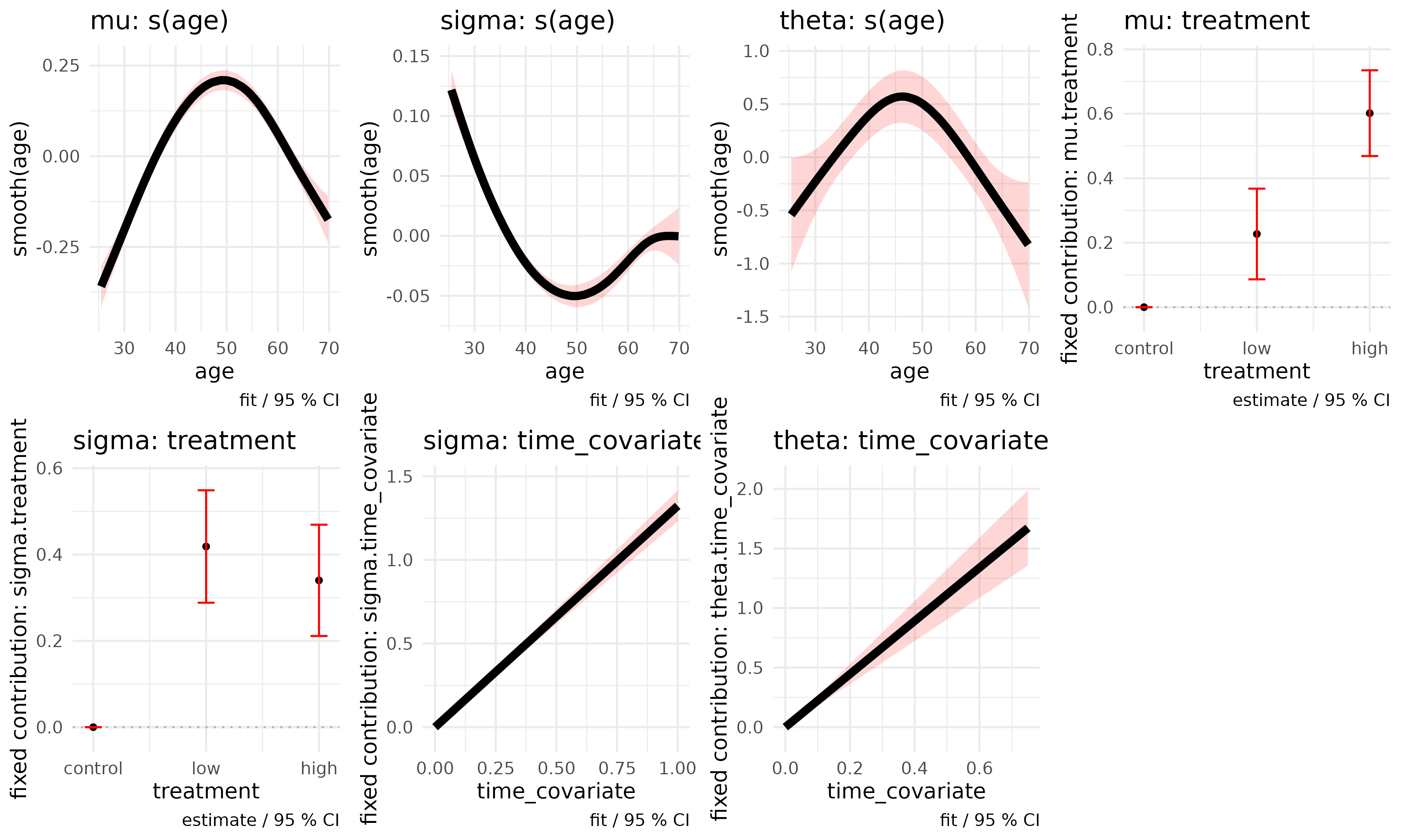

Key visual diagnostics are available using plot() for marginal diagnostics and plot_copula_diagnostics() for dependence diagnostics.

plot(fit)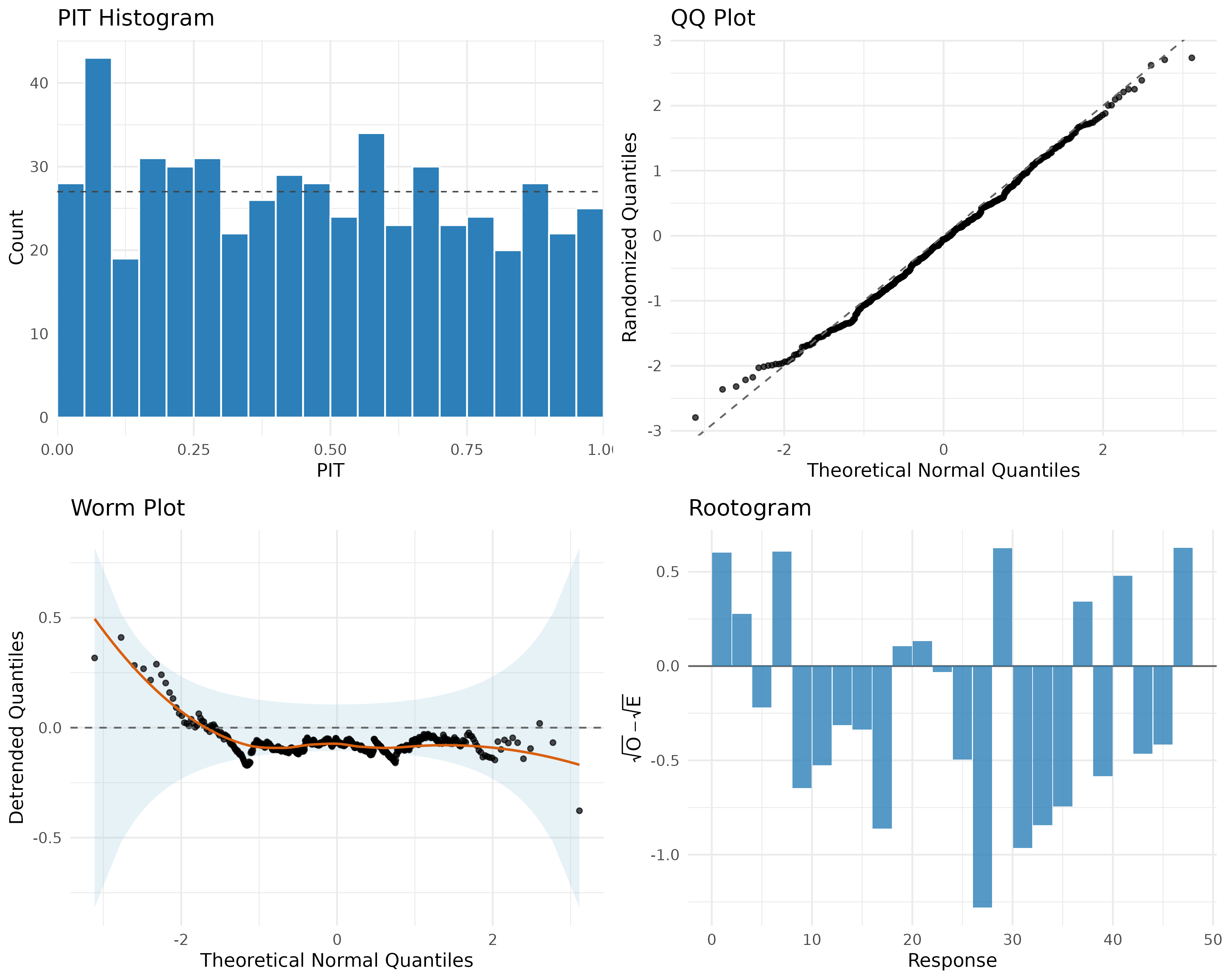

We will briefly comment on each of the marginal diagnostics and expected shape, though broadly they appear reasonable except some deviation in fit in the lower tail of the distribution.

Marginal diagnostics:

PIT appears reonasably close to uniform, with small deviation in the lower tail, PIT KS passes in numerical checks
QQ plot is very close to diagonal except in very low tail, though deviation is small
Worm plot should be close to centre line without deviation, but we do see some deviation in the lower tail more clearly than we could see in the QQ plot
Rootogram seems generally centred around zero with no major trends or deviation spikes

plot_copula_diagnostics(fit)

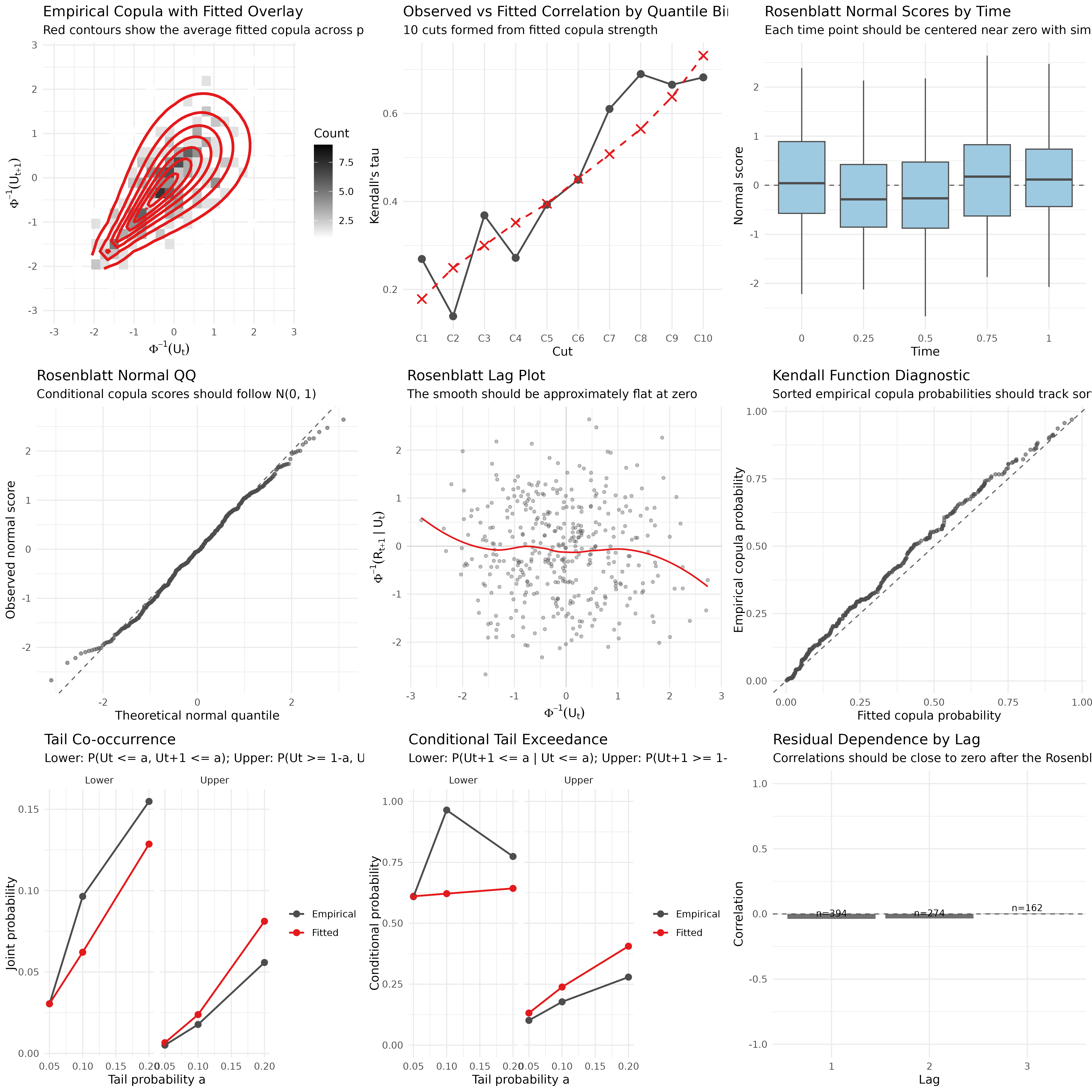
All trends for fitted versus observed dependence appear close. There is one small deviation between the fit and the data in the lower tail that can be seen in the Rosenblatt normal QQ plot and the tail co-occurrence / exceedence plots for the lower plot where we are slightly underfitting it appears.

We will briefly comment on each diagnostic for illustration purposes from left to right, then top to bottom:

Empirical copula overlay appears to broadly capture the shape of the 2d histogram, we can also plot the final fitted distributions against the original data using plot_margin_fit(fit, by_time=TRUE) and plot_copula_fit(fit, by_time=TRUE) if desired which will show the captured changing shape more clearly.
Deciles of fitted versus observed correlation follow the same trend indicating we are capturing the extremes and the centre of the correlation distribution (i.e. we are at least covering the range of correlation correctly)
Rosenblatt scores take into account correlation stucture in estimating residuals resulting in conditional estimates for margins, meaning they will tell us if the joint distribution (margin or copula) is misspecified. We provide multiple views:
- Rosenblatt z-scores by margin, which should be normally distributed at each time point (and are), a specific time point being non-normal indicates a specific set of copulas before it or the given margin is incorrectly specified
- Overall Rosenblatt Normal QQ plot indicates overall normality of the conditional residuals which look reasonable with small deviation in both tails
- Rosenblatt lag plot compares scores at a given time point with the lagged time point, which if correlation is correctly specified then these should be uncorrelated (and the are)
Kendall’s function diagnostic compares fitted copula probabilities across the dataset (sorted) against the empirical sorted copula probabilities and should follow the centre line without systematic deviation. In this case there is a small systematic deviation in the centre which may be worth investigating to improve the fit
Tail co-occurrence and exceedence compare empirical versus fitted probabiltiy of observations being in the upper and lower tails of the dependence structure and are broadly in line with some deviation in the lower tail, potentially due to the deviation in fit for the margin in the lower tail. This would indicate incorrectly specified tails either in the margin or the copula.
Residual dependence by lag should be close to zero if the copula is accurately capturing the dependence which it is here

Overall this appears to provide a reasonable fit to the joint distribution, with some small deviations in the tails for both the copula and margin which may warrant additional investigation.

Additional tools for inference, prediction, marginal effects, simulation, benchmarks

Standard functions for inference: confidence itervals, wald test, bootstrap

It’s straightforward to generate standard outputs for regression models such as confidence intervals and wald tests for coefficients of all parameters.

confint(fit)
#>                            2.5 %      97.5 %
#> theta.intercept      -0.69633689 -0.08903877
#> theta.time_covariate  1.80899030  2.65078222
#> nu.intercept          1.19195807  1.83596613
#> sigma.intercept      -1.36835951 -1.13561202
#> sigma.treatmentlow    0.28835742  0.54892519
#> sigma.treatmenthigh   0.21126445  0.46916845
#> sigma.time_covariate  1.22985542  1.41647908
#> mu.intercept          1.54676085  1.72816440
#> mu.treatmentlow       0.08639267  0.36762719
#> mu.treatmenthigh      0.46872278  0.73468394
wald_test(fit)
#> 
#> Wald Test for gamlss.longitudinal
#> ---------------------------------
#> Test type: individual 
#> VCOV method: analytical 
#> 
#>                  term estimate rhs std_error statistic    p_value     method
#>       theta.intercept  -0.3927   0   0.15493    -2.535  1.125e-02 analytical
#>  theta.time_covariate   2.2299   0   0.21475    10.384  2.939e-25 analytical
#>          nu.intercept   1.5140   0   0.16429     9.215  3.109e-20 analytical
#>       sigma.intercept  -1.2520   0   0.05938   -21.086  1.071e-98 analytical
#>    sigma.treatmentlow   0.4186   0   0.06647     6.298  3.016e-10 analytical
#>   sigma.treatmenthigh   0.3402   0   0.06579     5.171  2.328e-07 analytical
#>  sigma.time_covariate   1.3232   0   0.04761    27.792 5.359e-170 analytical
#>          mu.intercept   1.6375   0   0.04628    35.384 3.038e-274 analytical
#>       mu.treatmentlow   0.2270   0   0.07174     3.164  1.555e-03 analytical
#>      mu.treatmenthigh   0.6017   0   0.06785     8.868  7.424e-19 analytical

It’s also possible to produce bootstrap confidence intervals from the fitted model though it is computationally quite intensive as it refits the longitudinal model for each repetition (R=).

boot <- bootstrap_inference(
  fit,
  R = 5,
  seed = 20260521
)

print(boot)
#> 
#> Parametric Bootstrap for gamlss.longitudinal
#> -------------------------------------------
#> Replicates: 5 
#> Simulation: fitted copula model 
#> Failed refits: 0 
#> 
#>                  term estimate bootstrap_mean bootstrap_se conf.low conf.high
#>       theta.intercept  -0.3927        -0.3813      0.24633  -0.7479   -0.1549
#>  theta.time_covariate   2.2299         2.2305      0.22320   2.0355    2.5641
#>          nu.intercept   1.5140         1.6242      0.14792   1.4771    1.7859
#>       sigma.intercept  -1.2520        -1.2639      0.02191  -1.2801   -1.2299
#>    sigma.treatmentlow   0.4186         0.4288      0.05841   0.3417    0.4735
#>   sigma.treatmenthigh   0.3402         0.3316      0.07146   0.2604    0.4184
#>  sigma.time_covariate   1.3232         1.3087      0.04801   1.2451    1.3634
#>          mu.intercept   1.6375         1.6012      0.04296   1.5690    1.6679
#>       mu.treatmentlow   0.2270         0.2789      0.05739   0.2029    0.3352
#>      mu.treatmenthigh   0.6017         0.6379      0.07770   0.5516    0.7426
#>  reps
#>     5
#>     5
#>     5
#>     5
#>     5
#>     5
#>     5
#>     5
#>     5
#>     5

Benchmarking against standard models; gee, glmm, gam

It will be common for the user to be more familiar with longitudinal regression fits from a GEE using, for example, gee or geepack, or GLMM using mgcv or lme4. For ease of use, we provide the user a straightforward way to quickly compare a final model gamlss.longitudinal fit object to an alternative mean model using these frameworks with the same (or alternative) formula. First we can review a model with smooths which will only compare to mgcv based models (gam and gamm) which support smooths.

These comparison models should be treated as approximate or directional, as for a completely fair comparison the models selected for the benchmark comparison models should be (ideally) carefully selected within their own modelling framework rather than relying on the choices made for margin covariates made through the gamlss.longitudinal workflow.

The main idea of benchmark_standard_models is to provide a sense of the sensitivity of the model insights provided by gamlss.longitudinal (e.g. coefficients, confidence intervals, overall fit) to choice of model by directly comparing them to the alternative models.

We provide a bunch of metrics so that the user can decide the metrics of most importance to them. We initally present just a quick summary of the ‘best model’ by each dimension, then provide details of the metric values for each model fit as well as a detailed comparison of coefficients.

In general, we would expect that the mean-only models of GEEs and GLMMs will perform well when all three of these hold true: the primary question of interest is the value of the mean intercept, the marginal distribution is supported by the given models (generally exponential family), and the correlation structure is reasonably standard and does not rely on covariates strongly. If the question of interest relies on accurate confidence intervals or quantiles for parameters or predictions, and the distribution is non-exponential family, then the gamlss.longitudinal model is likely to perform better on metrics measuring those dimensions.

We group the benchmarking results into two groups: ‘Distributional’ which refers to metrics which measure the shape of the overall distribution where gamlss.longitudinal often performs better, e.g. log score, interval coverage, tail error / fit, and Mean fit which measures mean response, which benchmarked standard models are optimised against.

We see in both benchmark comparisons here that:

gamlss.longitudinal generally appears to provide the best fit by distributional fit including interval coverage, tail error and log score
glmer and gamm provide the best fits for MAE and RMSE against the observed response
Coefficients are broadly in the same ballpark between models, though there are significant differences, and, importantly, note the substantial differences in standard erros and therefore upper and lower 95% confidence intervals for parameters which are much tighter for the gamlss.longitudinal model due to the additional modelling of coefficients for both variance through sigma and nu and correlation through theta. Given coverage is more accurate for the gamlss.longitudinal model we could consider that these ranges may be more accurate, but much broader analysis is needed to confirm this (this work is in progress).

The selected final model does not include time on mu, while the benchmark mean model below does include a linear time term. To keep the selected final model unchanged while making the benchmark comparison like-for-like on the mean formula, we fit an additional comparison-only GAMLSS longitudinal model that adds time to mu and leaves the other final-model components unchanged.

fit_benchmark_mu_time <- gamlss_longitudinal(
  dataset = dataset,
  margin_dist = GG(),
  copula_dist = "C",
  time_var = "time",
  subject_var = "subject",
  mu.formula = response ~ treatment + time + s(age),
  sigma.formula = ~ treatment + time + s(age),
  nu.formula = ~ 1,
  theta.formula = ~ time + s(age)
)

bench <- benchmark_standard_models(
  data = dataset,
  formula = response ~ treatment + time + s(age),
  subject_var = "subject",
  family = "gamma",
  fit = fit_benchmark_mu_time,
  fit_name = "gamlss_long"
)
print(bench)
#> 
#> Standard Longitudinal Comparator Benchmark
#> -----------------------------------------
#> Formula: response ~ treatment + time + s(age) 
#> Subject: subject 
#> Family: Gamma 
#> Methods included: gamlss_long, gam, gamm 
#> Estimand note: mean-fit metrics compare response-mean predictions; distributional metrics use fitted quantiles, densities, PIT values, intervals, and tail probabilities where available.
#> 
#> Benchmark Summary
#> -----------------
#> 
#> Distributional
#> --------------
#>                   Metric  Best model
#>    95% interval coverage gamlss_long
#>       95% interval width        gamm
#>       Negative log score gamlss_long
#>           PIT KS p-value gamlss_long
#>  PIT mean absolute error        gamm
#>      Lower 5% tail error gamlss_long
#>      Upper 5% tail error gamlss_long
#> 
#> Mean fit
#> --------
#>                  Metric Best model
#>   Observed response MAE       gamm
#>  Observed response RMSE       gamm
#> 
#> Runtime
#> -------
#>              Metric Best model
#>  Elapsed time (sec)        gam
#> 
#> Benchmark Details
#> -----------------
#> Benchmark Metrics
#> -----------------
#>                   Metric gamlss_long        gam       gamm
#>       Elapsed time (sec)          NA  5.959e-02  5.257e-01
#>   Number of observations   6.000e+02  6.000e+02  6.000e+02
#>           Log likelihood  -1.107e+03 -1.449e+03 -1.345e+03
#>                      AIC   2.253e+03  2.914e+03  2.853e+03
#>                      MAE   3.571e+00  3.476e+00  2.737e+00
#>                     RMSE   5.306e+00  5.286e+00  4.548e+00
#>   Observed response RMSE   5.306e+00  5.286e+00  4.548e+00
#>    Observed response MAE   3.571e+00  3.476e+00  2.737e+00
#>       Negative log score   2.346e+00  2.691e+00  2.574e+00
#>    95% interval coverage   9.556e-01  9.185e-01  9.037e-01
#>       95% interval width   1.742e+01  2.138e+01  1.499e+01
#>  PIT mean absolute error   1.729e-02  1.863e-02  7.903e-03
#>           PIT KS p-value   2.553e-01  6.045e-04  7.440e-02
#>      Lower 5% tail error   7.407e-03  2.778e-02  3.519e-02
#>      Upper 5% tail error  -3.704e-03 -9.259e-03 -9.259e-03
#> 
#> Mu Coefficients
#> ---------------
#> Coefficient Estimates
#> 
#>           term gamlss_long      gam    gamm
#>      intercept      1.6761  1.81337  1.9578
#>   treatmentlow      0.2117 -0.08208 -0.2331
#>  treatmenthigh      0.5875  0.37371  0.2817
#>           time     -0.2119 -0.47957 -0.9781
#> 
#> Standard Errors
#> 
#>           term gamlss_long    gam    gamm
#>      intercept     0.04821 0.1079 0.12041
#>   treatmentlow     0.07366 0.1157 0.14434
#>  treatmenthigh     0.06837 0.1143 0.14160
#>           time     0.12924 0.1248 0.09839
#> 
#> 95% Lower Estimates
#> 
#>           term gamlss_long     gam      gamm
#>      intercept     1.58156  1.6019  1.721810
#>   treatmentlow     0.06729 -0.3088 -0.515955
#>  treatmenthigh     0.45349  0.1496  0.004122
#>           time    -0.46516 -0.7241 -1.170952
#> 
#> 95% Upper Estimates
#> 
#>           term gamlss_long     gam     gamm
#>      intercept     1.77055  2.0248  2.19382
#>   treatmentlow     0.35603  0.1447  0.04984
#>  treatmenthigh     0.72151  0.5978  0.55918
#>           time     0.04143 -0.2350 -0.78528

Then we can compare a reduced model without the age smooth to be able to compare all models. This is just illustrative so we remove the variable for simplicity, but you could alternatively group age or similar to be able to also compare this effect as well.

fit_reduced <- gamlss_longitudinal(
  dataset = dataset,
  margin_dist = GG(),
  copula_dist = "C",
  time_var = "time",
  subject_var = "subject",
  mu.formula = response ~ treatment,
  sigma.formula = ~ treatment + (time),
  nu.formula = ~ 1,
  theta.formula = ~ (time)
)
#> Missingness Summary (by time):
#>   time n_total n_na_response n_observed_response
#> 1 0.00     120             9                 111
#> 2 0.25     120             8                 112
#> 3 0.50     120            13                 107
#> 4 0.75     120            10                 110
#> 5 1.00     120            20                 100
#> 
#> Consecutive Pair Completeness:
#>   time1 time2 complete_pairs total_pairs total_observations
#> 1  0.00  0.25            103         120                600
#> 2  0.25  0.50            100         120                600
#> 3  0.50  0.75             98         120                600
#> 4  0.75  1.00             93         120                600
#> 
#> 
#> Running separate RS warm-start phase for 5 outer iteration(s) before joint RS fit...
#> 
#> Using automatic step_adjustment=1 for joint RS.
#> 
#> Using stop criteria: inner_stop_crit= 0.000229653 | outer_stop_crit= 0.00114827 
#> 
#> OUTER ITERATION: 1
#> Start LogLik   End LogLik       Change 
#> -1148.266279 -1145.301181     2.965098 
#> 
#> OUTER ITERATION: 2
#>  Start LogLik    End LogLik        Change 
#> -1.145301e+03 -1.145202e+03  9.891077e-02 
#> 
#> OUTER ITERATION: 3
#>  Start LogLik    End LogLik        Change 
#> -1.145202e+03 -1.145166e+03  3.637873e-02 
#> 
#> OUTER ITERATION: 4
#>  Start LogLik    End LogLik        Change 
#> -1.145166e+03 -1.145141e+03  2.446458e-02 
#> 
#> OUTER ITERATION: 5
#>  Start LogLik    End LogLik        Change 
#> -1.145141e+03 -1.145125e+03  1.641073e-02 
#> 
#> OUTER ITERATION: 6
#> Start LogLik   End LogLik       Change 
#> -1145.125016 -1145.114965     0.010051 
#> 
#> OUTER ITERATION: 7
#>  Start LogLik    End LogLik        Change 
#> -1.145115e+03 -1.145108e+03  7.205572e-03 
#> 
#> OUTER ITERATION: 8
#>  Start LogLik    End LogLik        Change 
#> -1.145108e+03 -1.145103e+03  4.528090e-03 
#> 
#> OUTER ITERATION: 9
#>  Start LogLik    End LogLik        Change 
#> -1.145103e+03 -1.145100e+03  3.393647e-03 
#> 
#> OUTER ITERATION: 10
#>  Start LogLik    End LogLik        Change 
#> -1.145100e+03 -1.145098e+03  2.302145e-03 
#> 
#> OUTER ITERATION: 11
#>  Start LogLik    End LogLik        Change 
#> -1.145098e+03 -1.145096e+03  1.660554e-03 
#> 
#> OUTER ITERATION: 12
#>  Start LogLik    End LogLik        Change 
#> -1.145096e+03 -1.145095e+03  1.110994e-03 
#>       joint 
#> 0.001110994 
#> 
#> OUTER CONVERGED
#> 
#> ############ MODEL FIT ############
#> 
#> Margin distribution: generalised Gamma Lopatatsidis-Green
#> Copula distribution: C
#> 
#> Parameter count: 10
#> Observations: 600
#> Margins: 5
#> 
#> Total time (seconds): 3.98
#> 
#>                        estimate
#> theta.intercept      -0.3161307
#> theta.time_covariate  1.9411706
#> nu.intercept          1.5839249
#> sigma.intercept      -1.1064279
#> sigma.treatmentlow    0.3213018
#> sigma.treatmenthigh   0.2293979
#> sigma.time_covariate  1.2219567
#> mu.intercept          1.6035303
#> mu.treatmentlow       0.3507522
#> mu.treatmenthigh      0.6852418
#> 
#> Model Selection Criteria:
#>         marginal    copula     joint
#> LogLik -1295.626  150.5314 -1145.095
#> AIC     2607.252 -297.0628  2310.190
#> BIC     2642.428 -288.2690  2354.159
#> EDF        8.000    2.0000    10.000
#> 
#> ####################################
#> Calculating variance-covariance matrix at fit completion...
#> Analytical Hessian: computing eta and likelihood components...
#> Analytical Hessian: computing CDF derivatives...
#> Analytical Hessian: assembling copula Hessian contributions...
#> Analytical Hessian: extracting margin second derivatives...
#> Analytical Hessian: assembling covariate Hessian matrix...
#> Analytical Hessian: done.

fit_reduced_mu_time <- gamlss_longitudinal(
  dataset = dataset,
  margin_dist = GG(),
  copula_dist = "C",
  time_var = "time",
  subject_var = "subject",
  mu.formula = response ~ treatment + time,
  sigma.formula = ~ treatment + (time),
  nu.formula = ~ 1,
  theta.formula = ~ (time)
)
#> Missingness Summary (by time):
#>   time n_total n_na_response n_observed_response
#> 1 0.00     120             9                 111
#> 2 0.25     120             8                 112
#> 3 0.50     120            13                 107
#> 4 0.75     120            10                 110
#> 5 1.00     120            20                 100
#> 
#> Consecutive Pair Completeness:
#>   time1 time2 complete_pairs total_pairs total_observations
#> 1  0.00  0.25            103         120                600
#> 2  0.25  0.50            100         120                600
#> 3  0.50  0.75             98         120                600
#> 4  0.75  1.00             93         120                600
#> 
#> 
#> Running separate RS warm-start phase for 5 outer iteration(s) before joint RS fit...
#> 
#> Using automatic step_adjustment=1 for joint RS.
#> 
#> Using stop criteria: inner_stop_crit= 0.000229218 | outer_stop_crit= 0.00114609 
#> 
#> OUTER ITERATION: 1
#> Start LogLik   End LogLik       Change 
#>  -1146.08790  -1144.16129      1.92661 
#> 
#> OUTER ITERATION: 2
#>  Start LogLik    End LogLik        Change 
#> -1.144161e+03 -1.144134e+03  2.722155e-02 
#> 
#> OUTER ITERATION: 3
#>  Start LogLik    End LogLik        Change 
#> -1.144134e+03 -1.144129e+03  5.556540e-03 
#> 
#> OUTER ITERATION: 4
#>  Start LogLik    End LogLik        Change 
#> -1.144129e+03 -1.144125e+03  3.790863e-03 
#> 
#> OUTER ITERATION: 5
#>  Start LogLik    End LogLik        Change 
#> -1.144125e+03 -1.144122e+03  2.886765e-03 
#> 
#> OUTER ITERATION: 6
#>  Start LogLik    End LogLik        Change 
#> -1.144122e+03 -1.144119e+03  2.450680e-03 
#> 
#> OUTER ITERATION: 7
#>  Start LogLik    End LogLik        Change 
#> -1.144119e+03 -1.144117e+03  2.026319e-03 
#> 
#> OUTER ITERATION: 8
#>  Start LogLik    End LogLik        Change 
#> -1.144117e+03 -1.144116e+03  1.484072e-03 
#> 
#> OUTER ITERATION: 9
#>  Start LogLik    End LogLik        Change 
#> -1.144116e+03 -1.144114e+03  1.417483e-03 
#> 
#> OUTER ITERATION: 10
#>  Start LogLik    End LogLik        Change 
#> -1.144114e+03 -1.144114e+03  9.281266e-04 
#>        joint 
#> 0.0009281266 
#> 
#> OUTER CONVERGED
#> 
#> ############ MODEL FIT ############
#> 
#> Margin distribution: generalised Gamma Lopatatsidis-Green
#> Copula distribution: C
#> 
#> Parameter count: 11
#> Observations: 600
#> Margins: 5
#> 
#> Total time (seconds): 2.29
#> 
#>                        estimate
#> theta.intercept      -0.3378273
#> theta.time_covariate  1.9489442
#> nu.intercept          1.4675518
#> sigma.intercept      -1.1062871
#> sigma.treatmentlow    0.3276979
#> sigma.treatmenthigh   0.2342655
#> sigma.time_covariate  1.2465622
#> mu.intercept          1.6287336
#> mu.treatmentlow       0.3315160
#> mu.treatmenthigh      0.6705071
#> mu.time_covariate    -0.1640275
#> 
#> Model Selection Criteria:
#>         marginal    copula     joint
#> LogLik -1293.535  149.4216 -1144.114
#> AIC     2605.070 -294.8431  2310.227
#> BIC     2644.643 -286.0493  2358.593
#> EDF        9.000    2.0000    11.000
#> 
#> ####################################
#> Calculating variance-covariance matrix at fit completion...
#> Analytical Hessian: computing eta and likelihood components...
#> Analytical Hessian: computing CDF derivatives...
#> Analytical Hessian: assembling copula Hessian contributions...
#> Analytical Hessian: extracting margin second derivatives...
#> Analytical Hessian: assembling covariate Hessian matrix...
#> Analytical Hessian: done.


bench <- benchmark_standard_models(
  data = dataset,
  formula = response ~ treatment + time,
  subject_var = "subject",
  family = "gamma",
  fit = fit_reduced_mu_time,
  fit_name = "gamlss_long"
)
print(bench)
#> 
#> Standard Longitudinal Comparator Benchmark
#> -----------------------------------------
#> Formula: response ~ treatment + time 
#> Subject: subject 
#> Family: Gamma 
#> Methods included: gamlss_long, glm, geeglm, glmer, gam, gamm 
#> Estimand note: mean-fit metrics compare response-mean predictions; distributional metrics use fitted quantiles, densities, PIT values, intervals, and tail probabilities where available.
#> 
#> Benchmark Summary
#> -----------------
#> 
#> Distributional
#> --------------
#>                   Metric   Best model
#>    95% interval coverage  gamlss_long
#>       95% interval width  glmer, gamm
#>       Negative log score  gamlss_long
#>           PIT KS p-value  gamlss_long
#>  PIT mean absolute error geeglm, gamm
#>      Lower 5% tail error  gamlss_long
#>      Upper 5% tail error  gamlss_long
#> 
#> Mean fit
#> --------
#>                  Metric  Best model
#>   Observed response MAE glmer, gamm
#>  Observed response RMSE glmer, gamm
#> 
#> Runtime
#> -------
#>              Metric Best model
#>  Elapsed time (sec)        glm
#> 
#> Benchmark Details
#> -----------------
#> Benchmark Metrics
#> -----------------
#>                   Metric gamlss_long        glm     geeglm      glmer
#>       Elapsed time (sec)          NA  3.133e-03   0.013626  2.260e-01
#>   Number of observations   6.000e+02  6.000e+02 600.000000  6.000e+02
#>           Log likelihood  -1.144e+03 -1.465e+03         NA -1.441e+03
#>                      AIC   2.310e+03  2.940e+03         NA  2.895e+03
#>                      MAE   3.753e+00  3.618e+00   3.647169  2.820e+00
#>                     RMSE   5.464e+00  5.428e+00   5.431785  4.696e+00
#>   Observed response RMSE   5.464e+00  5.428e+00   5.431785  4.696e+00
#>    Observed response MAE   3.753e+00  3.618e+00   3.647169  2.820e+00
#>       Negative log score   2.395e+00  2.716e+00   2.718878  2.557e+00
#>    95% interval coverage   9.481e-01  9.130e-01   0.914815  9.074e-01
#>       95% interval width   1.835e+01  2.149e+01  21.782363  1.499e+01
#>  PIT mean absolute error   2.394e-02  1.381e-02   0.007131  7.363e-03
#>           PIT KS p-value   1.743e-01  3.935e-03   0.018412  1.108e-01
#>      Lower 5% tail error   5.556e-03  2.593e-02   0.029630  3.704e-02
#>      Upper 5% tail error  -3.704e-03 -9.259e-03  -0.009259 -5.556e-03
#>         gam       gamm
#>   1.587e-02  4.203e-01
#>   6.000e+02  6.000e+02
#>  -1.460e+03 -1.343e+03
#>   2.930e+03  2.851e+03
#>   3.618e+00  2.775e+00
#>   5.428e+00  4.599e+00
#>   5.428e+00  4.599e+00
#>   3.618e+00  2.775e+00
#>   2.716e+00  2.576e+00
#>   9.130e-01  9.019e-01
#>   2.149e+01  1.481e+01
#>   1.381e-02  7.001e-03
#>   3.935e-03  8.771e-02
#>   2.593e-02  3.889e-02
#>  -9.259e-03 -9.259e-03
#> 
#> Mu Coefficients
#> ---------------
#> Coefficient Estimates
#> 
#>           term gamlss_long     glm   geeglm   glmer     gam    gamm
#>      intercept      1.6287  1.7755  1.79602  1.9681  1.7755  1.9315
#>   treatmentlow      0.3315  0.0156  0.01326 -0.1938  0.0156 -0.1739
#>  treatmenthigh      0.6705  0.4311  0.46396  0.3199  0.4311  0.3290
#>           time     -0.1640 -0.4678 -0.50017 -1.0985 -0.4678 -1.0090
#> 
#> Standard Errors
#> 
#>           term gamlss_long    glm  geeglm  glmer    gam    gamm
#>      intercept     0.05569 0.1070 0.09509 0.1669 0.1070 0.12261
#>   treatmentlow     0.08319 0.1142 0.15061 0.1970 0.1142 0.14757
#>  treatmenthigh     0.07740 0.1128 0.14070 0.1921 0.1128 0.14458
#>           time     0.14090 0.1248 0.12906 0.1391 0.1248 0.09742
#> 
#> 95% Lower Estimates
#> 
#>           term gamlss_long     glm  geeglm    glmer     gam     gamm
#>      intercept      1.5196  1.5658  1.6096  1.64104  1.5658  1.69115
#>   treatmentlow      0.1685 -0.2083 -0.2819 -0.57992 -0.2083 -0.46309
#>  treatmenthigh      0.5188  0.2101  0.1882 -0.05655  0.2101  0.04561
#>           time     -0.4402 -0.7123 -0.7531 -1.37111 -0.7124 -1.19998
#> 
#> 95% Upper Estimates
#> 
#>           term gamlss_long     glm  geeglm   glmer     gam    gamm
#>      intercept      1.7379  1.9851  1.9824  2.2952  1.9852  2.1718
#>   treatmentlow      0.4946  0.2395  0.3085  0.1923  0.2395  0.1154
#>  treatmenthigh      0.8222  0.6521  0.7397  0.6964  0.6521  0.6124
#>           time      0.1121 -0.2233 -0.2472 -0.8258 -0.2233 -0.8181

Prediction and simulation

All standard prediction options are available as part of the predict() method for gamlss.longitudinal fit objects, see help("predict.gamlss.longitudinal") for all options. We also provide a standard method to replicate the known method often used for mixed models margins_effects so that average predictions across a variable can be provided.

Note that the NA here for the reponse for row 4 and 6 are from the original data

# Predict the fitted response mean with confidence interval
pred=predict(
  fit,
  newdata = dat,
  type = "mean",
  se.fit = TRUE,
  interval = "confidence"
)
head(pred)
#>   subject time   response      fit    se.fit conf.low conf.high
#> 1       1 0.00 14.0634049 8.600757 0.4841117 7.651915  9.549598
#> 2       1 0.25 12.7321135 8.300118 0.4841117 7.351277  9.248960
#> 3       1 0.50  5.3841679 7.803959 0.4841117 6.855117  8.752800
#> 4       1 0.75         NA 7.087139 0.4841117 6.138297  8.035980
#> 5       1 1.00  0.2474735 6.209750 0.4841117 5.260908  7.158591
#> 6       2 0.00         NA 7.189700 0.4495594 6.308580  8.070820

# Calculate average response across a covariate for the margin
meff=marginal_effects(
  fit,
  newdata = dat,
  variable = "treatment",
  parameter = "mu",
  se.fit = TRUE
)
head(meff)
#>    variable   value parameter estimate   std_error reference contrast conf.low
#> 1 treatment control        mu 5.208493 0.009957978   control 0.000000 5.188976
#> 2 treatment     low        mu 6.535838 0.016181980   control 1.327345 6.504121
#> 3 treatment    high        mu 9.506673 0.021227317   control 4.298180 9.465068
#>   conf.high
#> 1  5.228010
#> 2  6.567554
#> 3  9.548277

We also provide standard functionality for simulating from the fitted model which uses the copula structure to create margins which are correlated as would be expected based on the fitted copula.

sim_model <- simulate(fit, nsim = 5, seed = 1)
head(sim_model)
#>       sim_1      sim_2        sim_3        sim_4      sim_5
#> 1  6.143973  7.3152724 6.7935658377  9.503653475 11.1621032
#> 2  5.334784 17.2903970 5.7528920106  9.251484936 19.3140574
#> 3  5.749883 13.0858360 7.1554217799 13.099713890  9.7002136
#> 4        NA         NA           NA           NA         NA
#> 5 19.605728  0.3872792 0.0001055938  0.004956788  0.2090253
#> 6        NA         NA           NA           NA         NA

Final remarks

Thanks for reviewing our detailed worked example.

gamlss.longitudinal is a work in progress. If you are working with our package and come across any issues, please drop them into our github page https://github.com/ahibbert/gamlss.longitudinal/issues or reach out to the author and we’ll get back to you as soon as we can. We appreciate your assistance in helping us improve gamlss.longitudinal for everyone!